Distributions

Introduction

Picking a probability distribution to represent your emissions data is a necessary step to calculating a UPL, regardless of the method you use or any other parameters you change. If you are using the frequentist methods behind Normal_UPL(), Lognormal_UPL(), and Skewed_UPL(), than you are picking the distribution based on ratios of skewness and kurtosis and it is explicitly assumed to be correct in the UPL calculations. If you are using the Bayesian_UPL() method, then you can compare as many distributions as you like and choose the best based on quantitative and qualitative comparisons to the actual observation density. At the moment, the UPLforOAR package supports Beta, Gamma, Lognormal, Normal, and Skewed for Bayesian_UPL(). However, there are many more distributions already supported in R and JAGS (also known as BUGS, a slightly different version of the same software). This vignette describes the supported distributions and links to resources for more that can be included in future development as needed. Much of the content on distributions comes from either BUGS documentation or the reference book “Bayesian Models: A Statistical Primer for Ecologists” by N. Thompson Hobbs and Mevin B. Hooten, Princeton University Press 2015.

Beta

The Beta distribution models random variables that can only take on values between 0 and 1. It is often used for probabilities and proportions, and is a good choice to consider for emissions variables that are represented as destruction or removal efficiencies. The probability density, $p(x)$, of Beta distributed emissions, $x$, is dependent on parameters $\alpha$ and $\beta$:

$$p(x) = \frac{\Gamma(\alpha + \beta)}{\Gamma(\alpha)\Gamma(\beta)}x^{\alpha -1}(1-x)^{\beta-1}$$

Note that $\Gamma$ in this case is the gamma function not the Gamma probability distribution. Using moment-matching, you can calculate the mean and variance of the Beta distribution as:

$$\mu = \frac{\alpha}{\alpha + \beta},~~ \sigma^{2} = \frac{\alpha \beta}{(\alpha + \beta)^{2}(\alpha + \beta +1)}$$

The parameters $\alpha$ and $\beta$ can be positive and negative, though shouldn’t be able to take on values below -1. In JAGS the distribution is defined as $\sim dbeta(\alpha, ~\beta)$.

Gamma

The Gamma distribution is very useful for emissions data because it represents strictly positive skewed continuous data. The probability density, $p(x)$, of Gamma distributed emissions, $x$, is dependent on parameters shape, $\alpha$, and rate, $\beta$:

$$p(x) = \frac{\beta^{\alpha}}{\Gamma(\alpha)}x^{\alpha-1}e^{-\beta x}$$

Note that $\Gamma$ in this case is the gamma function not the Gamma probability distribution. Both the shape and rate must be positive real numbers. Using moment-matching, you can calculate the mean and variance of the Gamma distribution as:

$$\mu = \frac{\alpha}{\beta},~~\sigma^{2} = \frac{\alpha}{\beta^{2}}$$

In JAGS the distribution is defined as $\sim dgamma(\alpha, ~\beta)$.

Lognormal

If a variable $z$ is Normally distributed, then $e^z$ is Lognormally distributed. If a variable $x$ is Lognormally distributed, than a variable $log(x)$ is Normally distributed. The product of large numbers of random variables is Lognormally distributed regardless of the distributions of the individual variables. It is often used to model growth or products of states or parameters. It is continuous and strictly positive, and can be asymmetric, which can be well suited to describe emissions data. The probability for the Lognormal distribution is dependent on parameters $\mu$, the mean of $log(x)$ and $\sigma$, the standard deviation of $log(x)$:

$$p(x) = \frac{1}{x\sqrt{2\pi \sigma^{2}}}e^{-\frac{(log(x)-\mu)^{2}}{2\sigma^2}}$$

Using moment-matching, you can calculate the mean and variance of the Lognormal distribution as: $$mean = e^{\mu+\sigma^2/2}, ~~variance = (e^{\sigma^2}-1)e^{2\mu+\sigma^2}$$

Note that the variance and mean are interdependent, which makes the Lognormal particularly useful in cases where the variance of the data increases with the mean. In JAGS the distribution is defined as $\sim dlnorm(\mu, ~\frac{1}{\sigma^{2}})$. Note that rather than variance like R uses, JAGS takes the precision as the second input. There is no analytical solution for the arithmetic mean of future samples from the Lognormal distribution, so the UPL has to be calculated using an approximation in Lognormal_UPL() based on Gram-Charlier Series-A expansion (for more details see “An upper prediction limit for the arithmetic mean of a lognormal random variable” by Dulal Kumar Bhaumik and Robert David Gibbons, 2004.). Using the Bayesian methods in Bayesian_UPL(), the UPL can be calculated the same as it would be for any distribution; by drawing the future samples from the posterior distributions. Given that the Lognormal distribution is often heavy-tailed, and that the 99^th UPL is by definition going to be in that tail, the distribution will often need to be truncated by some upper bound such that emissions beyond it unreasonable to consider. See the section below on heavy and long tailed distributions for more information.

Normal

The Normal distribution applies to continuous random variables across the entire number line, and has been widely used in statistics because it has properties allowing many results to be derived analytically. In addition, because the sum of a large number of samples from any distribution will be normally distributed, there are many situations it is suited to. However, the Normal distribution is not often a good choice for emissions data, which tend not to be symmetric, are strictly positive, and the variance is often related to the mean. The probability density, $p(x)$, of Normally distributed emissions, $x$, is dependent on parameters mean, $\mu$, and standard deviation, $\sigma$:

$$p(x) = \frac{1}{\sigma \sqrt{2\pi}}e^{-\frac{(x-\mu)^{2}}{2\sigma^{2}}}$$

In JAGS the distribution is defined as $\sim dnorm(\mu, ~\frac{1}{\sigma^{2}})$. Note that rather than variance like R uses, JAGS takes the precision as the second input. Since the mean and variance can be solved for analytically, Normal_UPL() uses these fixed-point estimates to calculate the UPL based on the desired number of future samples and significance. The Bayesian method employed in Bayesian_UPL() will arrive at the same estimates of mean, variance, and UPL, but will incorporate uncertainty in the mean and variance and offers more ways to evaluate if the Normal distribution is the best choice to represent the data.

Skewed

The Skewed or skew-normal distribution is a generalization of the Normal distribution that allows for skewness. As such, it also exists the entire number line, but it is not symmetric. The Skew-normal distribution is defined by three parameters; location $\xi$, scale $\omega$, and skewness $\alpha$. This equivalent to a Normal distribution when $\alpha = 0$, it is right-skewed if $\alpha > 0$, and left-skewed if $\alpha < 0$. The probability density, $p(x)$, of Skewed distributed emissions is:

$$p(x) = \frac{2}{\omega}\phi \left(\frac{x-\xi}{\omega}\right) \Phi \left(\alpha\left(\frac{x-\xi}{\omega}\right)\right)$$

Where $\phi(x)$ is the standard normal probability distribution, and $\Phi(x)$ is its cumulative probability distribution function, and $x$ is transformed to $\frac{x-\xi}{\omega}$. This can be expanded to:

$$p(x) = \frac{2}{\omega}\frac{1}{\sqrt{2\pi}}e^{-\frac{\left(\frac{x-\xi}{\omega}\right)^{2}}{2}}\frac{1}{2}\left[1+\frac{2}{\sqrt{\pi}}\int_0^{\alpha\frac{x-\xi}{\omega\sqrt{2}}}e^{-t^2}dt\right]$$

Unlike the Normal distribution, there is no closed-form expression for $\alpha$, $\xi$, and $\omega$. The method of moments can be used for approximations when sample skewness is not too large, which is useful for determining initial values for MCMC chains for these parameters, but not as a solution for parameterization. Since there is no analytical solution, the approach in Skewed_UPL() uses iterative shifting of the t-score until the desired significance is achieved.

The Skew-normal distribution is not included in JAGS, but it is in R via the sn package. However, any distribution can be coded manually in JAGS by using the ‘zero poisson’ method. This approach is equivalent to any standard distribution in how the parameters are solved for using MCMC and posterior distributions are returned. The main difference in implementation is that for the standard distributions already defined in JAGS, we can draw the ‘future’ samples and probability density at any emission observation value from within JAGS, whereas with a manually defined distribution like Skew-normal we need to use the posterior distributions of $\xi$, $\omega$, and $\alpha$ to define the probability density in R using sn::dsn() and take those future draws using sample(). There is no difference in results either way as long as we are controlling for stochasticity.

Long- and Heavy-Tailed Distributions

Some probability distributions, for example some Lognormal, can have long or heavy tails. This means that there is some tiny probability of extreme values that can occur, and the range of these extreme values, i.e. the tail, can be very long. Where exactly the tail ends is quite uncertain because we usually don’t have any data supporting the probability estimates along these tails. The vast majority of the probability and emission values are in the body of the distribution, which is well supported by the parameter estimates and data. To put it another way, you can have very similar mean and standard deviations defining two Lognormal distributions, and the bulk of their probability density curves will be very similar, but the extent of the tails might be quite different. Furthermore, any method that involves a stochastic component in solving for parameters (for example MCMC in JAGS) can end up with very different extents of the tails due to randomness, rather than as a result of process or data. While we can control the randomness to have exactly reproducible results, we still want the stochastic component of any Bayesian method to be minuscule in its contribution to the final result.

This matters quite a lot when the UPL is the 99^th percentile of a long-tailed distribution, because it is going to be within that tail. The UPL of a long-tailed distribution, whether it’s solved for using Bayesian_UPL() or Lognormal_UPL(), can end up being unrealistically large. Sometimes the 99^th percentile of a long-tailed distribution will be past the range of all emissions data, not just the top performers used to calculate the UPL, and sometimes it might be beyond what is physically possible. These are obvious situations where the UPL of such a long-tailed distribution should not be used, and either a different distribution should be used or measures should be taken to truncate the tail to physically reasonable bounds. This is done by default in Bayesian_UPL() with an upper limit of 3 times the maximum emissions value in the training data, but can be adjusted by setting maxY. Any distribution that does not have an unsupported long-tail will be unaffected by this setting.

Example

Let’s look at an example using HCl emissions from Lime processing. First we will load the data and use the Excel workbook methods to pick a distribution and calculate the UPL.

dat_emiss = read.csv("Lime_data.csv")
distr_choice = distribution_type(data = dat_emiss)
UPL_excel = Lognormal_UPL(data = dat_emiss)

The emissions are a Lognormal distribution with a corresponding UPL of 2.57 (Lb/ton of stone fed Lime). Next we will plot the density of the emission observations along with the corresponding Lognormal probability density distribution to see how it looks.

ggplot()+
  geom_line(data = obs_den_df, size=0.75,
            aes(y = ydens, x = x_hat, color = 'a'))+
  geom_area(data = obs_den_df, alpha=0.25,
            aes(y = ydens, x = x_hat, fill = 'a'))+
  geom_point(aes(y = ydens, x = emissions), data = Obs_onPoint,
             size = 3, alpha = 0.5, shape = 19, color = 'black')+
  geom_line(aes(y = pdf_ln, x = x_hat, color = 'c'),
               data = pred_dat, size = 0.75, linetype = 3)+
  geom_area(aes(y = pdf_ln, x = x_hat, fill = 'c'), alpha = 0.25,
            data = pred_dat)+
  ylab("Density")+xlab("HCl emissions (lb/ton stone fed lime)")+
  ggtitle("Excel-based distribution and UPL")+
  pop_distr_theme()+
  geom_vline(aes(xintercept = UPL_excel, color = 'c'), 
             linewidth = 1, linetype = 1)+
  scale_x_continuous(expand = expansion(mult = c(0, 0.05)))+
  scale_y_continuous(expand = expansion(mult = c(0, 0.05)))+
  coord_cartesian(clip = 'off')+
  labs(color = 'Density:', fill = 'Density:')+
  geom_rug(sides = 'b', aes(x = emissions), data = dat_emiss,
           alpha = 0.5, outside = TRUE, color = 'black')+
  scale_color_manual(values = c('black', '#FF7F00'),
                     labels = c('Observations', 'Lognormal'))+
  scale_fill_manual(values = c('black', '#FF7F00'),
                    labels = c('Observations', 'Lognormal'))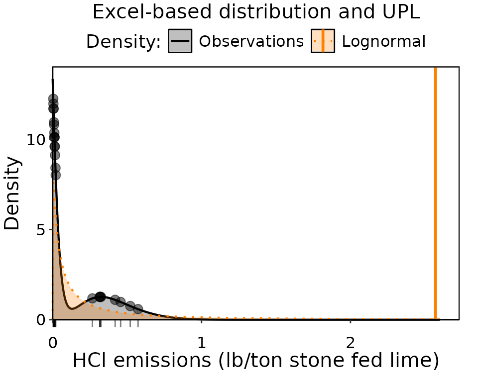

Observation density of HCl emissions. The obseration data are indicated in black as points and a rug along the axis, with the observation density distribution as a black line. The fitted lognormal distribution that is the basis of the UPL estimate is colored orange. The UPL result is the vertical orange line.

It is clear why the distribution is Lognormal over Normal or Skewed, since is a high density of very low emissions near zero that needs to be accommodated by the probability density distribution. However, it has a very long tail that results in an unreasonably large UPL that is 4.5 times larger than the largest emission. Instead, we will use a Bayesian approach that can do a better job representing the emissions.

Again with Bayes

Normally we would investigate multiple distributions because it is possible that a Gamma or a Beta might be better than the Lognormal and not have such a long tail. But for the sake of demonstrating how the tail affects the UPL, we will stick with the Lognormal. The methods in Bayesian_UPL() allow you to set a value at which to truncate the upper limit of emission probabilities, called maxY. By default, this is 3*max(data$emissions). We will also look setting maxY to 2*max(data$emissions) and 25*max(data$emissions) to see how the UPL estimate changes.

results_3X = Bayesian_UPL(distr_list = c("Lognormal"), data = dat_emiss,
                          xvals = seq(0, 3, length.out = 1000))
results_2X = Bayesian_UPL(distr_list = c("Lognormal"), data = dat_emiss,
                          maxY = 2*max(dat_emiss$emissions),
                          xvals = seq(0, 3, length.out = 1000))
results_25X = Bayesian_UPL(distr_list = c("Lognormal"), data = dat_emiss,
                           maxY = 25*max(dat_emiss$emissions),
                           xvals = seq(0, 3, length.out = 1000))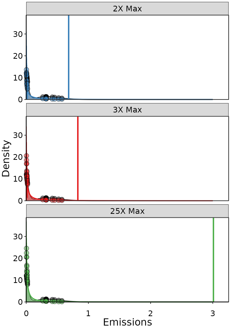

Example of three Lognormal distributions fit to the same data, but with different maximum emission thresholds.

Clearly, the longer the tail the larger the UPL: when the tail limit increases from 1.15, to 1.72, and then 5.74 we get UPL estimates of 0.68, 0.83, and 3.01. However, not all of these results are equal in terms of performance.

Let’s look at the results from fit_likelihood() to evaluate which distribution did a better job representing the actual observations. The distribution with the lowest upper limit of 1.15 did the best at actually fitting the data: it has the lowest SSE and the most observations within the 95% CI around predicted probability densities. The next higher limit had as many observations in agreement but a higher SSE. Lastly, the distribution with an extremely high upper limit that is unlikely to cause any truncation of probabilities, has the worst fit in terms of substantially higher SSE and more than half of the observations are outside the 95% CI on predicted density. Note that in all cases the area under the curve sums to less than 1, but the more the probability density function is truncated, the farther below 1.

Performance of Lognormal distributions with different MaxY limits

Upper Limit	UPL	SSE	No. Obs. in 95% CI	pdf integral
2X Max	0.68	110	15	0.65
3X Max	0.83	190	15	0.86
25X Max	3.00	570	10	0.93

Next we ought to check the convergence of all of the parameters. The model with maxY = 3*max(data$emissions) has one parameter with weak convergence according to the Gelman-Rubin diagnostics, so we will want to check all of the convergence figures. Issues with convergence can indicate that a distribution is not a good choice to represent the emissions data. The parameters technically passed the Gelman-Rubin diagnostic checks for all of them. However, for the 2X and 3X limits they do not look as well mixed as we would like, and you can see the histograms aren’t as Gaussian as can expect with good convergence. It is not so bad as to invalidate the results, but you can imagine that if we tried limits that were too small the model would fail.

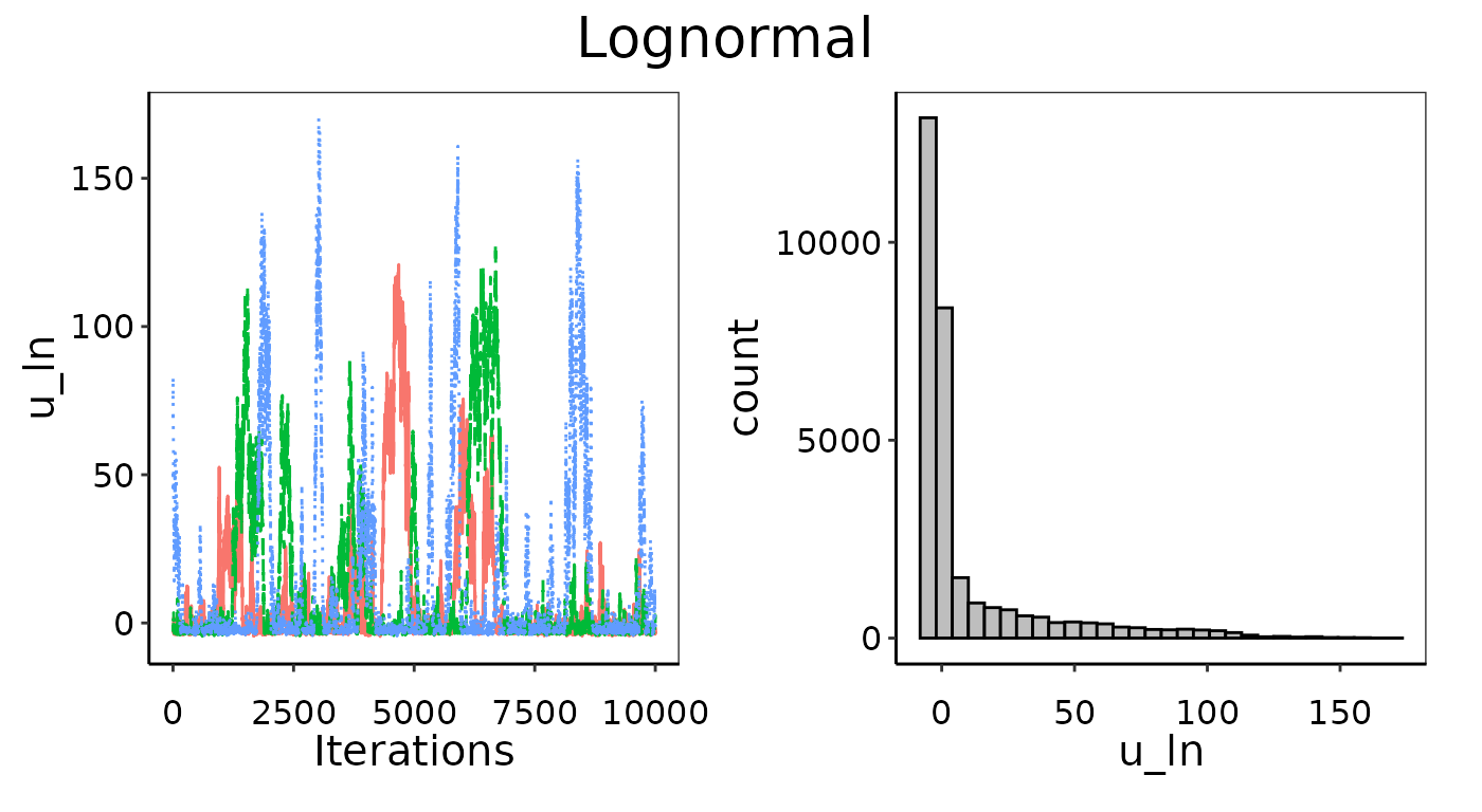
Convergence figures from maxY = 2X.

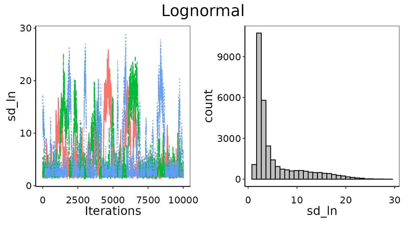
Convergence figures from maxY = 2X.

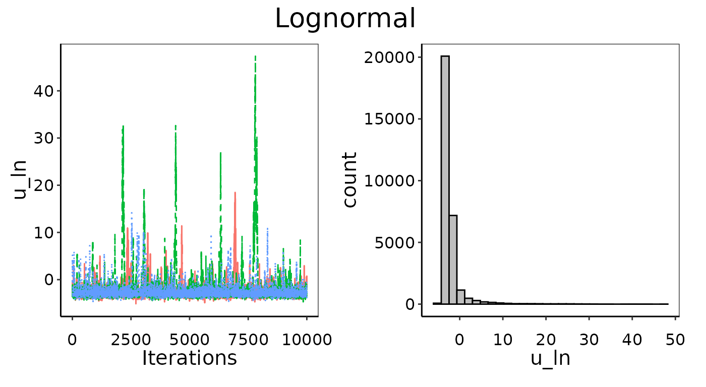
Convergence figures from maxY = 3X.

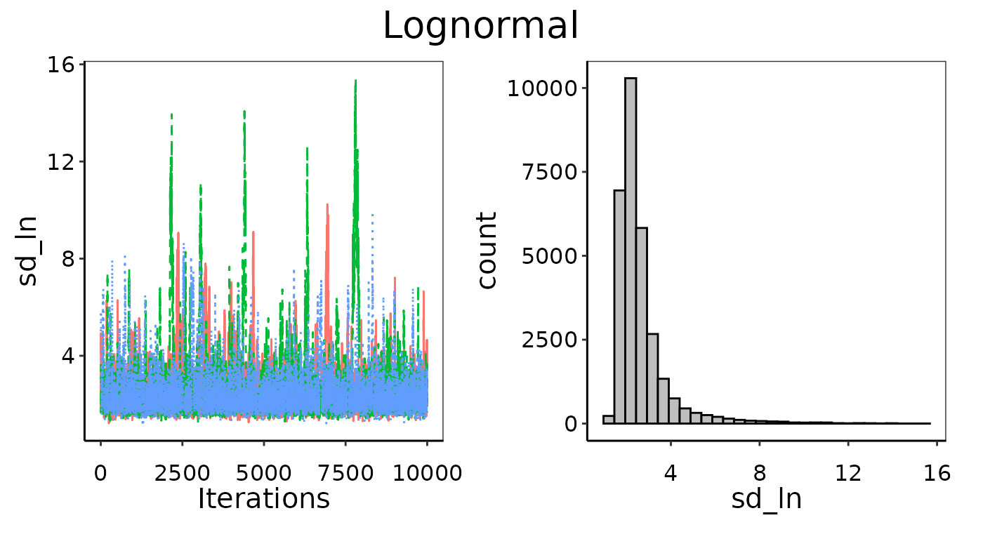
Convergence figures from maxY = 3X.

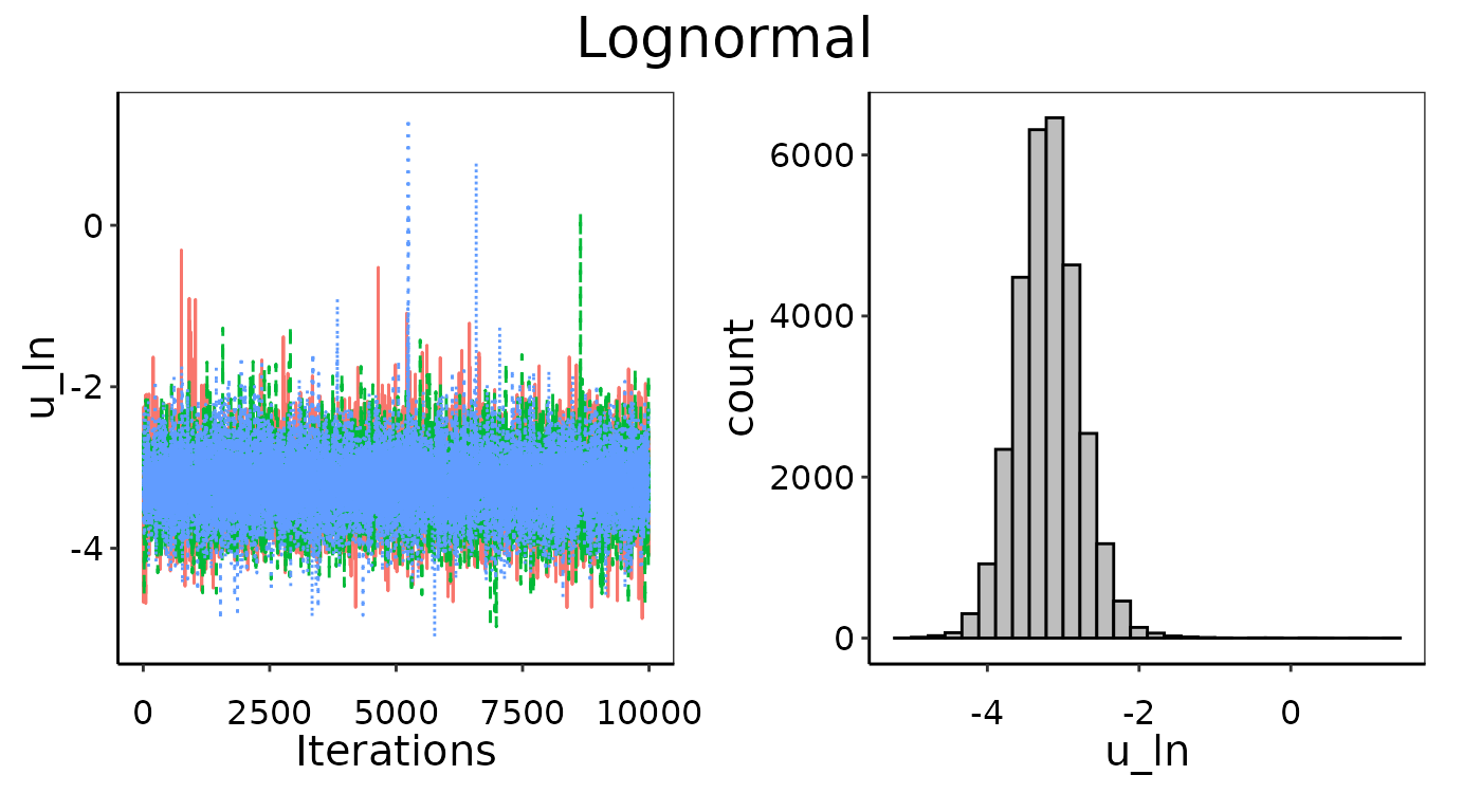
Convergence figures from maxY = 25X.

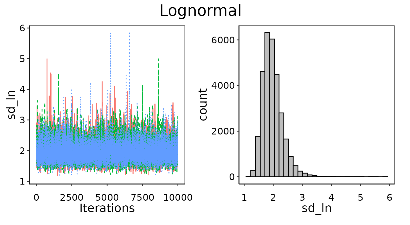
Convergence figures from maxY = 25X.

Picking an appropriate upper limit for maxY might not be an easy choice, and you should always vary it to check if you think your UPL results are in an unsupported long-tail. The alternative to using maxY to truncate the probability distribution is to use a different significance level. One that is lower than 0.99 might not be sensitive to the tail, and will be much less affected by u ncertainty and stochasticity in the tail of the distribution.

Alternative significance levels

Let’s investigate the sensitivity of different UPL significance levels to maxY. Ideally we will find a level that is insensitive to maxY and converges well.

results_3X95 = Bayesian_UPL(distr_list = c("Lognormal"), data = dat_emiss,
                            significance = 0.95,
                            xvals = seq(0, 3, length.out = 1000))
results_2X95 = Bayesian_UPL(distr_list = c("Lognormal"), data = dat_emiss,
                            significance = 0.95,
                            maxY = 2*max(dat_emiss$emissions),
                            xvals = seq(0, 3, length.out = 1000))
results_25X95 = Bayesian_UPL(distr_list = c("Lognormal"), data = dat_emiss,
                            maxY = 25*max(dat_emiss$emissions),
                            significance = 0.95,
                            xvals = seq(0, 3, length.out = 1000))
results_3X90 = Bayesian_UPL(distr_list = c("Lognormal"), data = dat_emiss,
                            significance = 0.90,
                            xvals = seq(0, 3, length.out = 1000))
results_2X90 = Bayesian_UPL(distr_list = c("Lognormal"), data = dat_emiss,
                            significance = 0.90,
                            maxY = 2*max(dat_emiss$emissions),
                            xvals = seq(0, 3, length.out = 1000))
results_25X90 = Bayesian_UPL(distr_list = c("Lognormal"), data = dat_emiss,
                             significance = 0.90,
                             maxY = 25*max(dat_emiss$emissions),
                             xvals = seq(0, 3, length.out = 1000))
results_3X85 = Bayesian_UPL(distr_list = c("Lognormal"), data = dat_emiss,
                            significance = 0.85,
                            xvals = seq(0, 3, length.out = 1000))
results_2X85 = Bayesian_UPL(distr_list = c("Lognormal"), data = dat_emiss,
                            significance = 0.85,
                            maxY = 2*max(dat_emiss$emissions),
                            xvals = seq(0, 3, length.out = 1000))
results_25X85 = Bayesian_UPL(distr_list = c("Lognormal"), data = dat_emiss,
                             significance = 0.85,
                             maxY = 25*max(dat_emiss$emissions),
                             xvals = seq(0, 3, length.out = 1000))
results_3X80 = Bayesian_UPL(distr_list = c("Lognormal"), data = dat_emiss,
                            significance = 0.80,
                            xvals = seq(0, 3, length.out = 1000))
results_2X80 = Bayesian_UPL(distr_list = c("Lognormal"), data = dat_emiss,
                            significance = 0.80,
                            maxY = 2*max(dat_emiss$emissions),
                            xvals = seq(0, 3, length.out = 1000))
results_25X80 = Bayesian_UPL(distr_list = c("Lognormal"), data = dat_emiss,
                             significance = 0.80,
                             maxY = 25*max(dat_emiss$emissions),
                             xvals = seq(0, 3, length.out = 1000))

The fitted probability density distribution won’t change with significance level, just the resulting UPL. The figure below shows the same distributions as before with the different maxY limits, but now we’ve added the UPL when calculated using 80%, 85%, 90%, 95% and 99% significance as vertical lines. As expected, lower significance has a lower UPL. The important outcome here is that at 80% and 85% significance the UPL doesn’t change no matter how we vary maxY. The UPL changes slightly at the highest maxY for 90%, and quite a lot as we increase maxY for 95% and 99% significance.

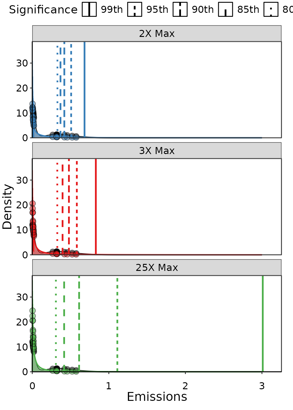
Example of three Lognormal distributions fit to the same data, but with different maximum emission thresholds and levels of significance. THe significnace only changes the UPL outcome, and each level has a different line type as a vertical line at the UPL.

Based on these results, we would conclude that at 85% significance the UPL is stable with regards to long-tail effects in the distribution. It is also worth pointing out that this area of the distribution also has data underlying it, increasing our confidence. Adjusting the significance to a stable level or changing maxY distribution limits are both ways to handle the unstable nature of long-tailed distributions, but both have draw backs. The best path forward is to avoid using UPL’s from long-tailed distributions all together. If you have a similar or almost as good fit to another distribution without the tail that will be a better choice for the UPL. You can always test the sensitivity to find out if your fitted distribution has a problematic tail by varying maxY across a range of high values outside your data as we did in this demo. Fundamentally, the 99^th percentile of a long tail is an unrealistic emission value. If no other distributions can be fit without a long tail, than the issue is likely a lack of representative data. More data will always go a long ways towards improving the distribution fit, and a lack of data can lead to one weird point forcing bad behavior.

Performance of Lognormal distributions with different MaxY limits and different significance levels.

Upper Limit	UPL	SSE	No. Obs. in 95% CI	pdf integral	Significance
2X Max	0.33	110	15	0.65	80th
3X Max	0.33	190	15	0.86	80th
25X Max	0.31	570	10	0.93	80th
2X Max	0.37	110	15	0.65	85th
3X Max	0.40	190	15	0.86	85th
25X Max	0.42	570	10	0.93	85th
2X Max	0.42	110	15	0.65	90th
3X Max	0.48	190	15	0.86	90th
25X Max	0.61	570	10	0.93	90th
2X Max	0.51	110	15	0.65	95th
3X Max	0.58	190	15	0.86	95th
25X Max	1.10	570	10	0.93	95th

Alternative distributions

Logically the next step is to try other distributions and see if we can find something better. We won’t bother with the Normal distribution since the data are so heavily skewed. We also won’t look at the Beta distribution since it has an upper limit of 1, and while the emissions observations are all less than that in our set of top performing sources, theoretically there could emissions higher than 1.

distributions = c('Gamma', 'Lognormal', 'Skewed')
results = Bayesian_UPL(data = dat_emiss, distr_list = distributions)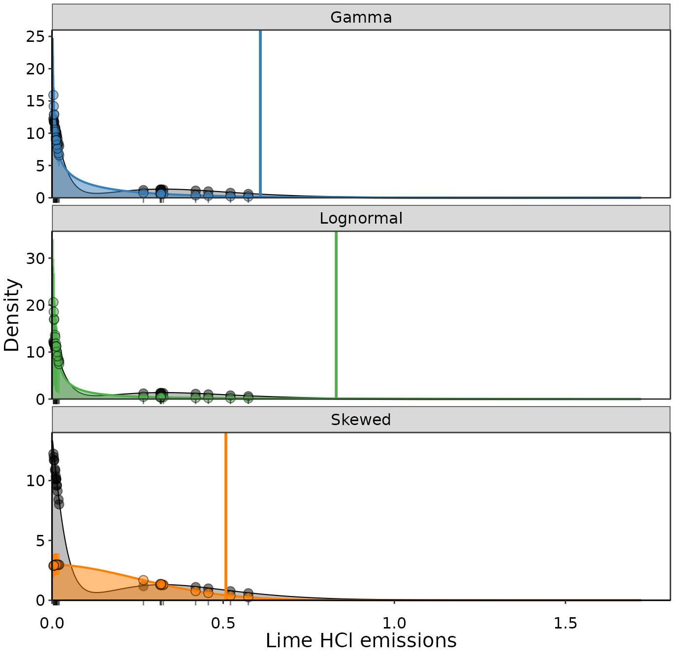

Fitted likelihood distributions for Lime HCl emissions.

fit_metrics = results$fit_table

Comparing goodness of fit results for other distributions

Distribution	UPL	SSE	No. Obs. in 95% CI	integral
Gamma	0.609	40.9	15	0.8966921
Lognormal	0.830	194.0	15	0.8558586
Skewed	0.508	840.0	4	0.9450102

The Gamma distribution looks the best and also has the lowest SSE. Furthermore, the Gamma distribution converges well. It still has a bit of a tail so we might want to repeat our experiments with increasingly larger values of maxY:

results_3X = Bayesian_UPL(distr_list = c("Gamma"), data = dat_emiss,
                          xvals = seq(0, 3, length.out = 1000))
results_2X = Bayesian_UPL(distr_list = c("Gamma"), data = dat_emiss,
                          maxY = 2*max(dat_emiss$emissions),
                          xvals = seq(0, 3, length.out = 1000))
results_25X = Bayesian_UPL(distr_list = c("Gamma"), data = dat_emiss,
                           maxY = 25*max(dat_emiss$emissions),
                           xvals = seq(0, 3, length.out = 1000))

The outcome shows the tail is way more stable at the 99^th percentile for Gamma than it was for Lognormal. Furthermore, the fit is just as good (SSE barely changes) and the UPL hardly changes. This is all great news, and leads us to finally recommend a UPL of 0.66.

Performance of Gamma distributions with different MaxY limits

Upper Limit	UPL	SSE	No. Obs. in 95% CI	pdf integral
2X Max	0.54	43	15	0.87
3X Max	0.61	41	15	0.87
25X Max	0.66	41	15	0.87