Convergence and Priors • UPLforOAR

Introduction

This vignette provides further details on convergence and prior distributions for Bayesian_UPL(). We recommend already having some familiarity with using the default settings of Bayesian_UPL() and working through the examples in vignette("Bayesian-UPL") before reading further.

Convergence

Convergence of distribution parameters is assessed quantitatively using the Gelman-Rubin diagnostic and qualitatively by producing figures in a convergence report pdf document.

The diagnostics are available in the $conv_output table from Bayesian_UPL() or from using converge_likelihood() directly on the results of run_likelihood(). There are several variables in the conv_output table: the distribution as distr, its corresponding parameters in params, the diagnostic in gelman_diag, and if it converged in convYN. For example, a Normal distribution will have both mean and standard deviation parameters in the table, where as a Gamma distribution will have shape and rate. For gelman_diag less than 1.1, the outcome is "Yes" it converged in convYN. For diagnostic values between 1.1 and 1.2 it is "Weak convergence", and "No" convergence for values greater than 1.2.

Problems: Failing Gelman-Rubin diagnostic

Things have to go really wrong for the Gelman-Rubin diagnostics to fail. You can fail these checks if you do not have a long enough number of iterations in the burn-in or a long enough number of kept iterations. However Bayesian_UPL() is set up so that the 10,000 iterations for burn-in and sampling should be sufficient as long as the likelihood model is somewhat reasonable. The diagnostic also relies on comparing multiple MCMC chains with substantially different initial values, which again is handled automatically in Bayesian_UPL(). Below is an example where we generated 30 random emissions between 0 and 100 and then tried to fit a Lognormal likelihood distribution. Unsurprisingly, it fails to converge.

set.seed(1)
emissions = runif(30, min = 0, max = 100)
results = Bayesian_UPL(distr_list = c("Lognormal"),
                       data = tibble(emissions = emissions))
conv_metrics=results$conv_output

Gelman-Rubin convergence tests for likelihood parameters
Distribution	Parameter	Diagnostic	Converged
Lognormal	u_ln	1.344	No
Lognormal	sd_ln	1.329	No

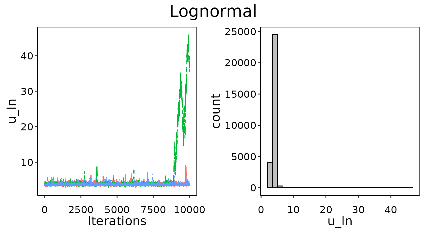
We can take a look at the figures generated in the convergence report as well. Note that for both parameters, the left figures show one of the chains is off on a tangent and they are clearly not well-mixed or without trend. This is the kind of behavior that will result in the Gelman-Rubin diagnostic failing.

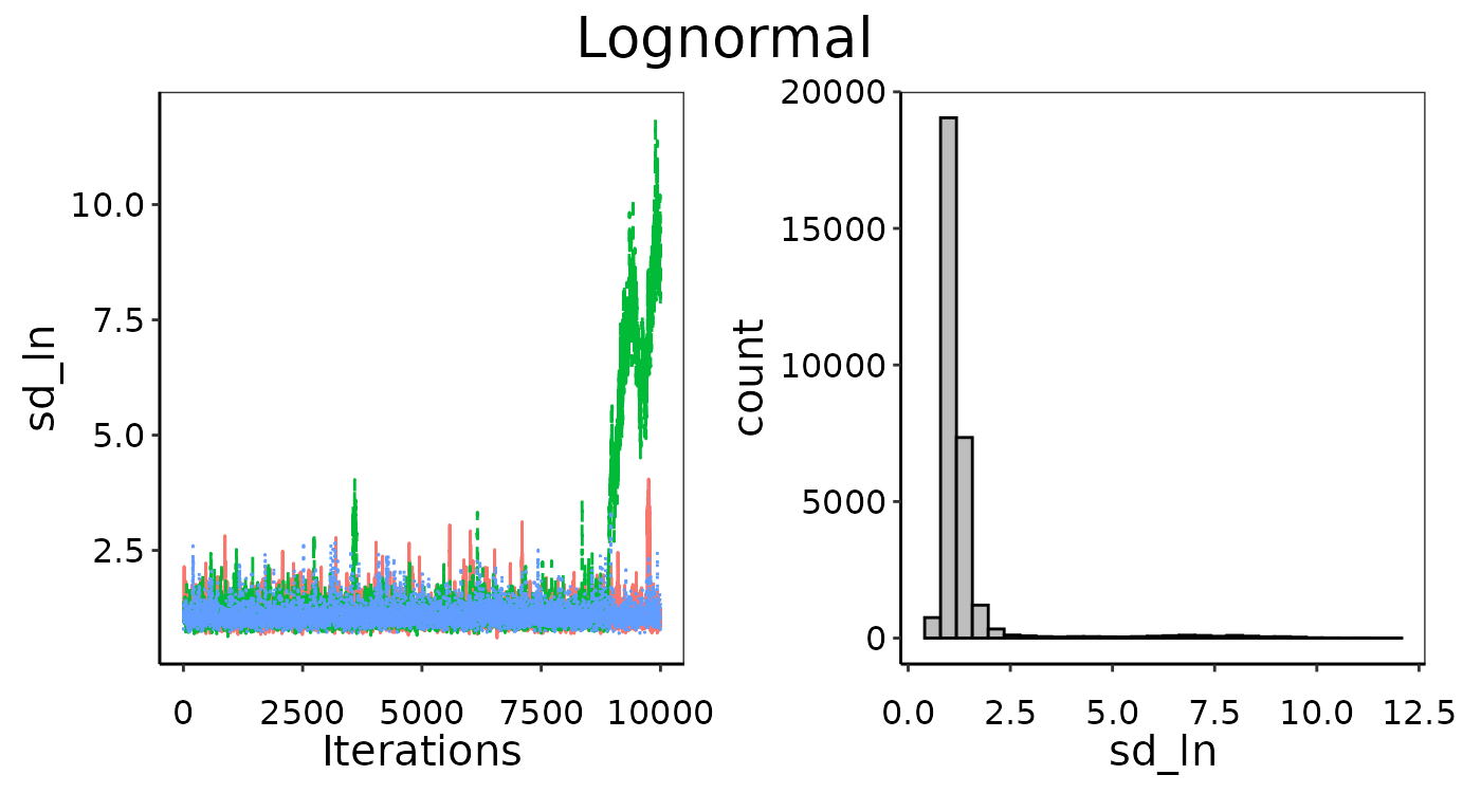
Example of bad convergence in MCMC chains.

It is possible for a parameter to pass the Gelman-Rubin test and indeed have chains well-mixed, but not arrive at a clear posterior distribution. That is why passing the Gelman-Rubin diagnostic is necessary but insufficient to indicate convergence. This can happen when there is too little data (for example extremely small data sets where n = 3), and the parameter posterior is simply returning the prior distribution. For example, a poorly converged Normal distribution might have an even probability of the mean being any emission value, in which case the histogram will be flat across the entire parameter-space.

Problems: Flat posterior

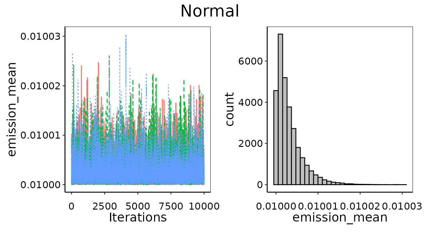
In the example below, we use only 3 observations used to fit a Normal distribution. This is as small a data set as one could conceivably use, and with only 3 runs there is not likely to be enough information to pick an appropriate distribution or determine its defining parameters with high confidence. Even though the Gelman-Rubin diagnostics passed in this case, and indeed the MCMC chains look well-mixed (left figures), it has not converged well. The histograms on the right show the posterior is too flat. Note that there is a slight peak for the emission_mean posterior around 0.01, which is indeed the average of the 3 points, but there is not enough information to definitely say this is much more likely than any other value searched.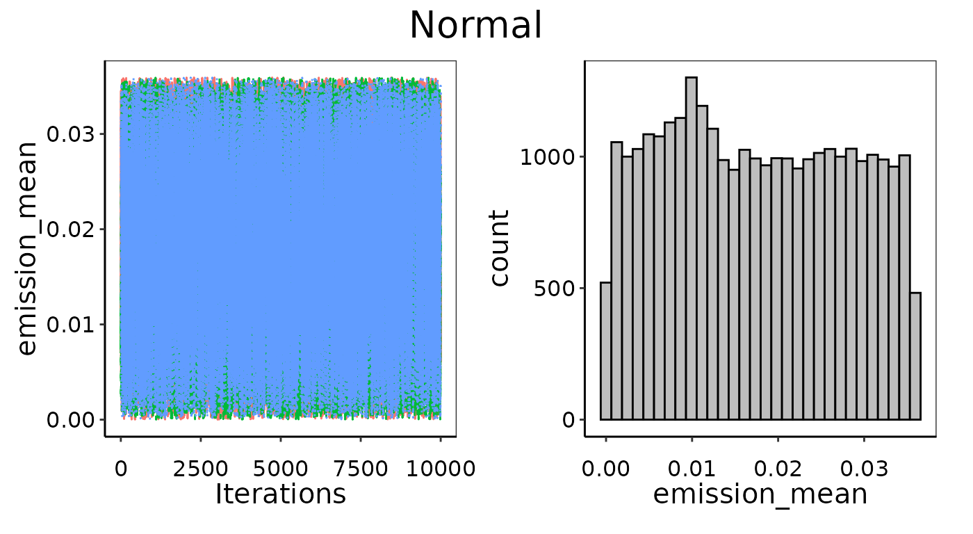

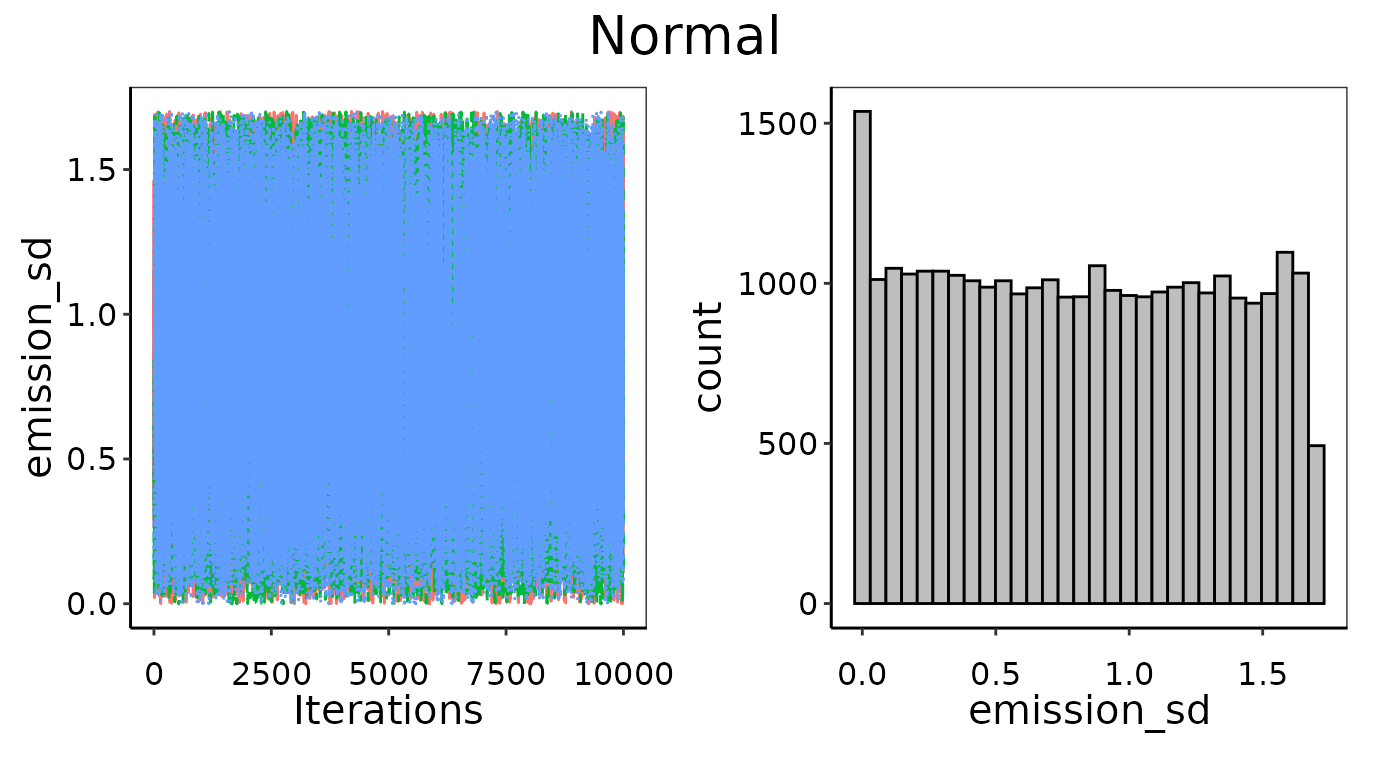
Example of bad convergence where posterior is too flat.

Problems: Bad prior limits

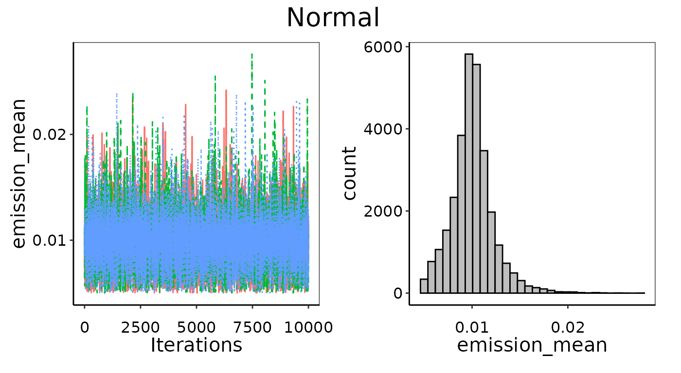
The visual assessment will also catch any issues with the prior distribution settings. Ideally, we are using uninformative priors for UPL calculations that have equal probability across a parameter-space that is much wider than the posterior result. This is determined automatically from the data, but in some cases that range might not wide enough. This will be apparent if the parameter’s posterior histogram is highly skewed towards the end of the allowed range. In this case, the priors will need to be set manually to a wider uninformative range. As an example, we’ve fit a Normal distribution to the HCl emissions from Integrated Iron and Steel but manually set the prior range so the mean is equally likely between ~dunif(0.01, 0.05). Given that the average emission is much lower than this range at 0.001, this is likely to cause issues for convergence even though it does pass the Gelman-Rubin checks. Even though the MCMC chains are well mixed, they are clearly stacking up against the lower bound and trying to converge on a lower mean than we have allowed. This skew in the chains (left) and histogram (right) indicate improper prior distribution bounds.

Example of bad convergence, where the prior limits are too restrictive.

Priors

Bayesian inference uses prior information to derive posterior distributions of model parameters. The default behavior in Bayesian_UPL() is to use uninformative priors which are calculated based on the range and variance of the emissions data. The prior information can be manually supplied to either increase the parameter space to search wider, or to provide more specific information, which might be particularly useful in circumstances where there are very few observations (i.e. n = 3).

It is inadvisable to use manual priors without good justification. A situation where one might use the manual prior option is after running Bayesian_UPL() with the default uninformative priors and the parameters showed issues with convergence. For example, if the posterior histogram is completely flat across the default parameter space, and information from the data are limited by a low sample size, then a narrower parameter range might need to be provided manually to promote convergence. Alternatively, if the posterior histogram appears to be stacked up along one side of the parameter space, then a wider prior range might need to be provided manually if applicable. Some parameters can only exist above 0, or -1, or between -1 and 1, and in these cases it is not abnormal behavior for their posterior distributions to be heavily skewed when close to a boundary, and setting further limits manually will not change any outcomes.

Manual limits on priors

In the convergence section above we tried to fit a Normal distribution to an emission data set with n = 3 and fully uninformed priors, and did not achieve good convergence. We could then decide to follow up with another Normal distribution where we provide slightly narrower but still largely uninformative priors manually. The first pair in prior_list are the bounds on standard deviation and encompass several orders of magnitude around the actual standard deviation of the 3 observations. The second pair of bounds in prior_list encompass the actual mean of 0.01, but aren’t quite as wide as the automated uninformative priors uses. This slight restriction on the prior search is enough to promote better convergence, as can be seen in the two resulting fitted probability density distributions below. Note that both have very large error bars around the probability density at the emission observations. This is expected given how little information we actually get from 3 observations. The ability to quantify this uncertainty is a nice outcome of using a Bayesian approach.

result_informed = Bayesian_UPL(distr_list = c("Normal"), data = small_dat,
                               manual_prior = TRUE,
                               prior_list = c(0.0001, 0.01, 0.005, 0.03))
result_uninformed = Bayesian_UPL(distr_list = c("Normal"), data = small_dat)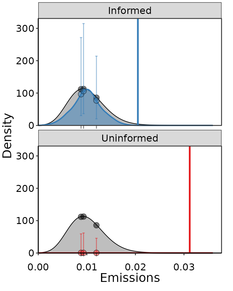

Example of two Normal distributions fit to the same 3 points of data, where one was more informative using slightly smaller bounds on prior distributions, and the other was completely uninformative and did not converge well.

We can look at how the convergence figures are different in the case where we provided slightly more prior information. Note that the histograms are much more converged than the flat horizontal coverage they were when using the automated uninformed priors. Even though we provided the prior distributions manually, they are still considered to be uninformative. We have restricted the parameter space with lower and upper bounds, but it is still a wide accommodation, and within that all parameter outcomes are equally likely before we consider the data.

Improved convergence of parameters by providing slightly more restrictive bounds as priors.

Specific priors

In some cases there might be specific prior information about the distributions that can be used to set informative priors. Examples could include an operational lower or upper limit to emissions that physically cannot be surpassed, or the results from a previous decade of emissions that technology has improved on since. Specific prior information could be in the form of an informative distribution, such as ~dnorm(5, 0.1), rather than lower and upper bounds. In this case, the JAGS model scripts created by write_likelihood() will need to be edited to reflect the specifically defined distributions. Caution should be exercised if using stricter priors, and needs to be very well justified.